Machine Learning projects consist of several distinct steps: first, data validation verifies the state of the collected data. Processing prepares the features so an algorithm can consume them. Model training makes learning feasible, and model validation guarantees generalization. Fine-tuning adjusts the hyper-parameters to obtain the optimum results. Finally, after numerous iterations, the last step deploys a model to staging or production.

Each of these steps can be a separate process, running at its own cadence, with well-defined inputs and outputs. Thus, data scientists and ML engineers tend to think of these projects like pipelines. If there is something wrong with incoming information, the process could fail or even worse corrupt downstream analytic tasks. Thus, standardizing the process of creating these interconnected actions can make the pipeline more robust.

In this article, we demonstrate how to turn Jupyter Notebooks into Kubeflow Pipelines and Katib Experiments automatically. Such a system eliminates the erroneous process of manually extracting the bits that make sense in a Notebook, containerize them and launching a Pipeline using explicit Domain-Specific Languages.

Setting Up Kubeflow

Kubeflow is an open-source project, dedicated to making deployments of ML projects simpler, portable and scalable. The goal here is not to recreate other services, but to provide a straightforward way to use and deploy the best open-source tools for ML on any Kubernetes-ready environment.

However, setting up a Kubeflow instance is not an easy task, especially if you have no experience with Kubernetes. But that shouldn’t stop anyone; MiniKF on Google Cloud Platform (GCP) and AWS provides a fast and straightforward way to get started with Kubeflow.

We can have a single-node cluster up and running in ten minutes by following the steps below:

1. Visit the MiniKF on GCP, or AWS, marketplace page and click Launch
2. Set the VM configuration and click Deploy*

The deployment takes up to ten minutes, and we can watch the progress by following the on-screen instructions; SSH into the machine, run minikf on the terminal and wait until MiniKF has your endpoint and credentials ready. When the script is completed we should see the Kubeflow Dashboard endpoint and our credentials in the screen, as shown in Figure 1.

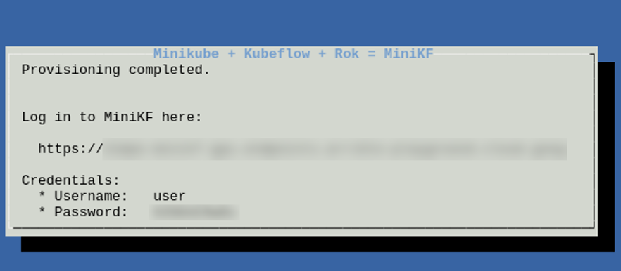
Figure 1 – Provision Completed

When the provision script is done, we are ready to visit the Kubeflow Dashboard by visiting the URL and entering our credentials, as shown in Figure 2.

On the left panel we can see that we have a lot of options. We can create Notebook servers, Volumes and run Pipelines and Katib experiments. To get started, we should create a Notebook server and start experimenting.

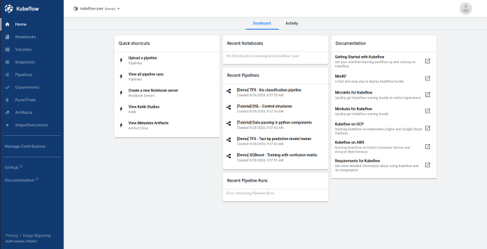
Figure 2 – Kubeflow Dashboard

Creating a Jupyter Server

Setting up a Jupyter Notebook is relatively easy in Kubeflow. We first need to create a Jupyter server and connect to it:

1. Choose Notebooks from the left panel
2. Click the New Server button on top
3. Fill in a name for the server and request the amount of CPU and RAM you need
4. Leave the Jupyter Notebook image as is — this is crucial for this tutorial**

After completing these four steps, we should wait for the Notebook Server to get ready and connect. After that we will be transferred to a familiar JupyterLab workspace.

From Jupyter to Kubeflow Pipelines

To transform a Jupyter Notebook into a Kubeflow Pipeline automatically, we use Kale. Kale is an open source tool that lets you deploy Jupyter Notebooks that run on your laptop or on the cloud to Kubeflow Pipelines, without requiring any of the Kubeflow SDK boilerplate. You can define pipelines just by annotating Notebook’s code cells and clicking a deployment button in the Jupyter UI. Kale will take care of converting the Notebook to a valid Kubeflow Pipelines deployment, resolving data dependencies and managing the pipeline’s lifecycle.

First, we need an example. So, let us clone the Kale repository and pick up one of the examples there.

This repository contains a series of curated examples with data and annotated Notebooks. Navigate to the folder data/kale/examples/dog-breed-identification/ in the sidebar and open the notebook dog-breed.ipynb.

To install the necessary dependencies run the cell following the imports and restart the notebook as shown in Figures 3.

Figure 3 – Install the Necessary Dependencies

We can skip running the cells that download the whole dataset and the bottleneck features. We are going to use the smaller samples that are included in the repository we just cloned.

On the left panel of the Notebook we see the Kale icon. Click it to enable the Kale extension. You will automatically see that every cell is annotated. The Notebook comes in sections; the imports, the data loading part, data processing, model training and evaluation, etc. This is precisely what is annotated by Kale. Now, this Notebook comes pre-annotated, but we can play around. We can create new pipeline steps, but we should not forget to add their dependencies.

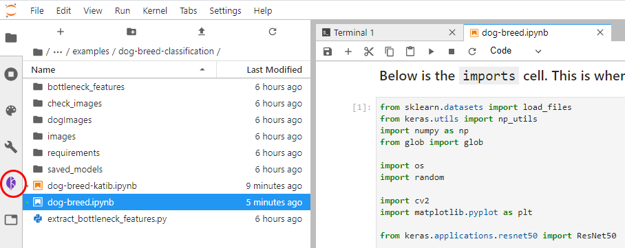
Figure 4 – Kale automation built into the UI

Figure 5 – Compile and Run the Notebook

In any case, we can click the Compile and Run button located at the bottom of the Kale Deployment Panel as shown in Figures 4 and 5. Without writing a single line of code, your Notebook will be transformed into a Kubeflow Pipeline, which will be executed as part of a new experiment.

Figure 6 – Compile and Run the Notebook

Follow the link provided by Kale as shown in Figure 6 to watch the running experiment. After a few minutes, the pipeline will complete its task successfully.

Watch the pipeline complete via the graph view highlighted in Figure 7.

Figure 7 – The Completed Pipeline

Hyper-Parameter Tuning

Creating a hyper-parameter (HP) tuning experiment using Kale and Katib, the HP Tuning component of Kubeflow, is likewise a simple click-and-run process. Back to the notebook server in your Kubeflow UI, launch the notebook named dog-breed-katib.ipynb. You are going to run some hyperparameter tuning experiments on the ResNet-50 model, using Katib. Notice that you have one cell in the beginning of the notebook to declare hyperparameters.

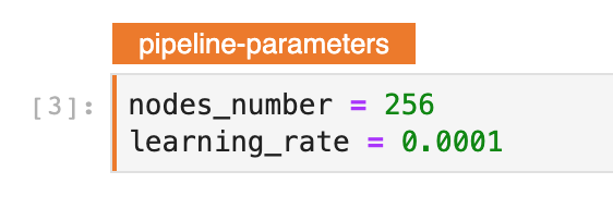
Figure 8 – Declaring the Hyper-Parameters

In the left pane of the notebook, enable HP Tuning with Katib and set up a job to run hyperparameter tuning, as shown in Figure 7.

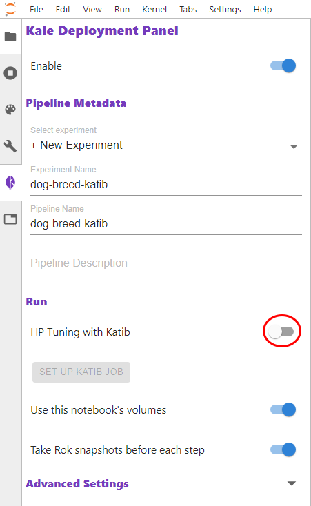
Figure 9 – Enable HP Tuning with Katib

We see that Kale auto-detects the HP Tuning Parameters and their type from the Notebook. This is possible due to the way we defined the parameters cell in the Notebook. In Figure 10, we define the search space for each parameter, and also set a goal.

Figure 10 – Setting Up a Katib Job

Like before click on the Compile and Run Katib Job button at the bottom of the Kale UI and follow the on screen instructions to monitor the experiment. We have successfully run an end-to-end ML workflow all the way from a Notebook to a reproducible multi-step pipeline with hyperparameter tuning, using Kubeflow (MiniKF), Kale, Katib and KF Pipelines.

Conclusion

In this article, we saw how we can launch a single-node Kubeflow instance using MiniKF, create a notebook server and convert a simple Jupyter Notebook to a reproducible multi-step pipeline with hyperparameter tuning, without writing any boilerplate code.

*For best performance, keeping the default VM configuration is recommended

** jupyter-kale:v0.5.0-47-g2427cc9 — Note that the image tag may differ

To learn more about containerized infrastructure and cloud native technologies, consider joining us at KubeCon + CloudNativeCon NA Virtual, November 17-20.